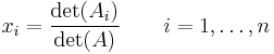
Determinant
In algebra, the determinant is a special number associated with any square matrix. The fundamental geometric meaning of a determinant is a scale factor for measure when the matrix is regarded as a linear transformation. Thus a 2 × 2 matrix with determinant 2 when applied to a set of points with finite area will transform those points into a set with twice the area. Determinants are important both in calculus, where they enter the substitution rule for several variables, and in multilinear algebra.
When its scalars are taken from a field F, a matrix is invertible if and only if its determinant is nonzero; more generally, when the scalars are taken from a commutative ring R, the matrix is invertible if and only if its determinant is a unit of R. Determinants are not that well-behaved for noncommutative rings.
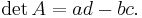
The determinant of a matrix A is denoted det(A), or without parentheses: det A. An alternative notation, used for compactness, especially in the case where the matrix entries are written out in full, is to denote the determinant of a matrix by surrounding the matrix entries by vertical bars instead of the usual brackets or parentheses. Thus
 denotes the determinant of the matrix
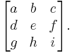
For a fixed nonnegative integer n, there is a unique determinant function for the n×n matrices over any commutative ring R. In particular, this unique function exists when R is the field of real or complex numbers.
The 2×2 matrix
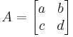
has determinant
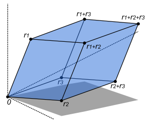
Interpretation as the area of a parallelogram
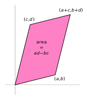
If A is a 2x2 matrix, its determinant det A can be viewed as the oriented area of the parallelogram with vertices at (0,0), (a,b), (a + c, b + d), and (c,d). The oriented area is the same as the usual area, except that it is negative when the vertices are listed in clockwise order.
Further, the parallelogram itself can be viewed as the unit square transformed by the matrix A. The assumption here is that a linear transformation is applied to row vectors as the vector-matrix product  , where
  is a column vector. The parallelogram in the figure is obtained by multiplying matrix A (which stores the co-ordinates of our parallelogram) with each of the row vectors
 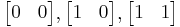 and
and  in turn. These row vectors define the vertices of the unit square. With the more common matrix-vector product
  the parallelogram has vertices at
 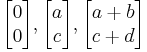 and
and  (note that
  ).
).
Thus when the determinant is equal to one, then the matrix represents an equi-areal mapping.
3-by-3 matrices
The determinant of a 3×3 matrix
is given by
- det (A) = aei + bfg + cdh − afh − bdi − ceg.

The rule of Sarrus is a mnemonic for this formula: the sum of the products of three diagonal north-west to south-east lines of matrix elements, minus the sum of the products of three diagonal south-west to north-east lines of elements when the copies of the first two columns of the matrix are written beside it as below:
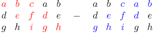
This mnemonic does not carry over into higher dimensions.
n-by-n matrices
The determinant of a matrix of arbitrary size can be defined by the Leibniz formula (as explained in the next paragraph) or the Laplace formula (as explained at the end of the Properties section).
The Leibniz formula for the determinant of an n-by-n matrix A is
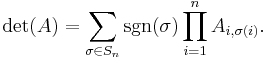
Here the sum is computed over all permutations σ of the numbers {1, 2, ..., n}. A permutation is a function that reorders this set of integers. For example, for n = 3, the original sequence 1, 2, 3 might be reordered to 2, 3, 1 or 3, 2, 1. It is a basic fact of combinatorics that there are n! = 1 · 2 · 3 · ... · n (n factorial) such permutations. The set of all such permutations is denoted Sn. For each permutation σ one computes the signature of σ; it is +1 for even and −1 for odd permutations. Evenness or oddness can be defined as follows: the permutation is even (odd) if the new sequence can be obtained by an even number (odd, respectively) of switches of adjacent numbers. For example, starting from 1, 2, 3 and switching once one gets 1, 3, 2, switching once more yields 3, 1, 2, and finally, after a total of three (an odd number) switches, one gets 3, 2, 1. Therefore this permutation is odd. The permutation 2, 3, 1 is even (1, 2, 3 → 2, 1, 3 → 2, 3, 1, two switches).
In any of the n factorial summands, the term

is a shorthand for the product over the indicated matrix entries, where i ranges from 1 to n, or equivalently:
For example, n = 4 and σ = (1, 4, 3, 2) yields sgn = -1 (three pair switches) and the matrix entries A11; A24; A33; A42. For small matrices, one gets back the formulae given in the previous sections.
The formal extension to arbitrary dimensions was made by Tullio Levi-Civita, see (Levi-Civita symbol) using a pseudo-tensor symbol. An alternative, but equivalent definition of the determinant can be obtained by using the following theorem:
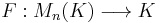
- Let Mn(K) denote the set of all
 matrices over the field K. There exists exactly one function
- with the two properties:
 is alternating multilinear with regard to columns;
 .
.
One can then define the determinant as the unique function with the above properties.
Determinant from LU decomposition
For matrices larger than 3x3 it is computationally cheaper (in number of operations conducted) to express, if possible,  , where P is a permutation matrix, L is a lower triangular matrix with diagonal elements equal to 1, and U is an upper triangular matrix. See LU decomposition for details on existence, uniqueness and algorithms for such a decomposition.
The determinant is then calculated as follows:

because  ; the right hand side is easily computed as the product of all diagonal elements of U multiplied with the determinant of the permutation matrix P (which is +1 for an even number of permutations and is -1 for an uneven number of permutations).
A small example:
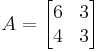
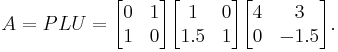
Therefore

Of course, for a 2-by-2 matrix the determinant is easily computed directly, 6 × 3 − 3 × 4 in this example, but for large matrices the LU decomposition produces significant computational savings: it reduces the number of operations from  for the Leibniz formula to
  .
.
Applications
Determinants are used to characterize invertible matrices (i.e., a matrix is invertible if and only if it has a non-zero determinant), and to explicitly describe the solution to a system of linear equations with Cramer's rule. This rule is denoted
where the matrix  is the matrix formed by the insertion of the solution column vector in the system of linear equations.
Determinants are useful to state solution properties. There are, however, much better numerical algorithms available to compute an inverse matrix and/or the solution of a system of linear equations, based on LU, QR, or singular value decomposition. These algorithms solve a linear equation system in O(n3), whereas Cramer's rule is O(n4).
Determinants can be used to find the eigenvalues of the matrix A through the characteristic polynomial
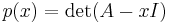
where I is the identity matrix of the same dimension as A.
Again, this formula is useful to state the properties of eigenvalues, but not to numerically compute them if n > 2. It is much more efficient and reliable to compute eigenvalues, e.g., with the QR algorithm.
One often thinks of the determinant as assigning a number to every sequence of  vectors in
  , by using the square matrix whose columns are the given vectors. With this understanding, the sign of the determinant of a basis can be used to define the notion of orientation in Euclidean spaces. The determinant of a set of vectors is positive if the vectors form a right-handed coordinate system, and negative if left-handed.
Determinants are used to calculate volumes in vector calculus: the absolute value of the determinant of real vectors is equal to the volume of the parallelepiped spanned by those vectors. As a consequence, if the linear map 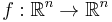 is represented by the matrix A, and
  is any measurable subset of , then the volume of
  is given by
 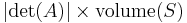 . More generally, if the linear map
 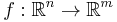 is represented by the
  -by- matrix A, and is any measurable subset of
  , then the -dimensional volume of is given by
 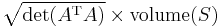 . By calculating the volume of the tetrahedron bounded by four points, they can be used to identify skew lines.
The volume of any tetrahedron, given its vertices a, b, c, and d, is (1/6)·|det(a − b, b − c, c − d)|, or any other combination of pairs of vertices that would form a spanning tree over the vertices.
Properties characterizing the determinant
In addition to the Leibniz formula above, there is another way of calculating determinants of matrices. It is based on the following properties of determinants:
- If A is a triangular matrix, i.e. Ai,j = 0 whenever i > j or, alternatively, whenever i < j, then
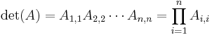 ,
,
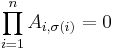 , for any permutation σ different from the identity permutation (the one not changing the order of the numbers 1, 2, ..., n)
 - If B results from A by interchanging two rows or two columns, then det(B) = −det(A).
- If B results from A by multiplying one row or column with a number c, then det(B) = c · det(A).
- If B results from A by adding a multiple of one row to another row, or a multiple of one column to another column, then
These four properties can be used to compute determinants of any matrix, using Gaussian elimination. This is an algorithm that transforms any given matrix to a triangular matrix, only by using the operations in the last three items. Since the effect of these operations on the determinant can be traced, the determinant of the original matrix is known, once Gaussian elimination is performed.
It is also possible to expand a determinant along a row or column using Laplace's formula, which is efficient for relatively small matrices. To do this along row  , say, we write
where the  represents the
  element of the matrix cofactors, i.e. is
  times the minor
  , which is the determinant of the matrix that results from A by removing the -th row and the
  -th column, and is the length of the matrix.
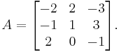
Example
The following compares various ways of calculating the determinant of the three-by-three matrix
| Method | Calculation | ||||||||||||
|---|---|---|---|---|---|---|---|---|---|---|---|---|---|
|
Rule of Sarrus |
|
||||||||||||
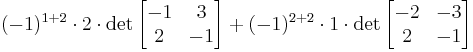
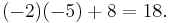
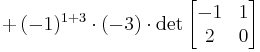
| Laplace expansion, along the second column (for ease of calculation, it is best to choose a row or column with many zeros)
In this case we see that j=2 and i will change as we move down the column. The last value will be zero and is not necessary to calculate (due to a 0 coefficient). |
|
||||||||||||
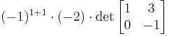
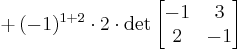
| Or, by using the first row: |
|
||||||||||||
| Gauss algorithm | 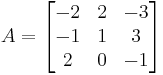
The determinant of the (upper) triangular matrix D is the product of its entries on the main diagonal: (−2) · 2 · 4.5 = −18. Therefore det(A) = +18. |


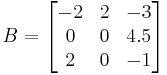 B is obtained from A by adding −1/2 × the first row to the second, so that det(A) = det(B)
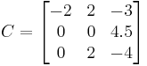 C is obtained from B by adding the first to the third row, so that det(C) = det(B)
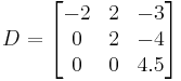 D is obtained from C by exchanging the second and third row, so that det(D) = −det(C)
Further properties
Basic properties
In this section all matrices are assumed to be n-by-n matrices.
The determinant of the identity matrix
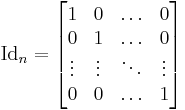
is one. This is even true if  , even though
  is an empty matrix.
The determinant is linear in each row of the matrix and also in each column of the matrix (in other words, when viewed as a function of the row of the matrix, the determinant is a multilinear map, and also when viewed as a function of the columns of the matrix). This means that if one fixes any row or column, and writes that row/column v of A as a linear combination of row/column vectors vk, then det(A) is equal to the same linear combination of the determinants of the matrices obtained from A by replacing v by vk while leaving all other entries unchanged. In particular, multiplying any individual row or column by r multiplies the determinant by r, and multiplying the entire matrix by r multiplies the determinant by rn.
The determinant is an alternating function of the rows of the matrix, and also of the columns of the matrix: whenever a matrix contains two identical rows or two identical columns, its determinant is 0. The rules given for the behaviour of the determinant under row and column operations follow from the multilinear and alternating properties. In fact the determinant can be characterized as the unique map from square matrices to scalars with the three properties listed so far.
The determinant of a rank-deficient matrix (one with rank less than n) is zero.
The determinant of a matrix product of square matrices equals the product of their determinants:
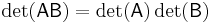
Thus the determinant is a multiplicative map. This formula is generalized by the Cauchy-Binet formula to (square) products of rectangular matrices.
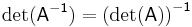
A matrix over a commutative ring R is invertible if and only if its determinant is a unit in R. In particular, if A is a matrix over a field, such as the real or complex numbers, then A is invertible if and only if det(A) is not zero. In this case
An important implication of the previous properties is the following: if A and B are similar, i.e., if there exists an invertible matrix X such that  , then

This means that the determinant is a similarity invariant. Because of this, the determinant of some linear transformation T : V → V for some finite dimensional vector space V is independent of the basis for V.
If A is triangular, then its determinant is the product of its diagonal entries.
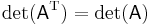
A matrix and its transpose have the same determinant:
The determinant is a natural transformation: for any ring homomorphism ƒ:R→S and any square matrix A with entries in R, the determinant of the matrix obtained by applying ƒ to each of the entries of A equals ƒ(det(A)). In particular, for complex matrices, the determinant of its complex conjugate matrix (or of its conjugate transpose) is the complex conjugate of its determinant. Another application of this property is for integer matrices: the reduction modulo m of the determinant of such a matrix is equal to the determinant of the matrix reduced modulo m (the latter determinant being computed using modular arithmetic).
If A is a square n-by-n matrix with real or complex entries, and if the characteristic polynomial splits into linear factors, then det(A) is the product of the eigenvalues of A, counted with their algebraic multiplicities.
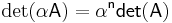
The determinant of a matrix multiplied by a scalar is:
Sylvester's determinant theorem
Sylvester's determinant theorem states that for A, an m-by-n matrix, and B, an n-by-m matrix,
 ,
,
where  and
and  are the m-by-m and n-by-n identity matrices, respectively.
For the case of column vector c and row vector r, each with m components, the formula allows the quick calculation of the determinant of a matrix that differs from the identity matrix by a matrix of rank 1:
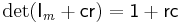 .
.
More generally, for any invertible m-by-m matrix X[1],
 ,
,
and
 .
.
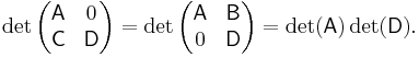
Block matrices
Suppose A, B, C, and D are n×n-, n×m-, m×n-, and m×m-matrices, respectively. Then
This can be seen from the Leibniz formula or by induction on n. When A is invertible, employing the following identity
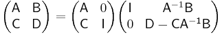
leads to
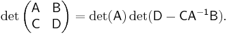
When D is invertible, a similar identity with  factored out can be derived analogously[2], that is,

Also[3],
When C and D commute, that is CD=DC, 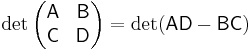 .
.
When A and C commute, that is AC=CA, 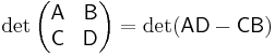 .
.
When B and D commute, that is BD=DB, 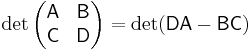 .
.
When A and B commute, that is AB=BA, 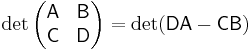 .
.
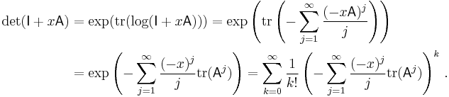
Relationship to trace
As mentioned above, the determinant equals the product of the eigenvalues. Similarly, the trace equals the sum of the eigenvalues. Thus,
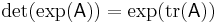
where  denotes the matrix exponential of
  , because every eigenvalue
  of corresponds to the eigenvalue
  of
of  .
.
Under the substitution ↦  , the matrix logarithm of , the above equation yields
 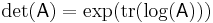 . Similarly,
 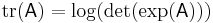 . The expression
  is closely related to the Fredholm determinant.
Size-specific relationships to trace
For an matrix , these formulae can be used to derive:


These formulae are closely related to Newton's identities.
Proof Outline
 is a polynomial in the variable , has degree at most , and the coefficient of
  is
is  . Working with
  small enough so that the power series for
  converges absolutely, we compute
Note that, despite appearances, each of these expressions simplifies to a polynomial of degree at most . In particular, it is safe to ignore all  terms, for
  . The coefficients of
  ,
,  ,
,  , and
, and  in this last expression give the above formulae.
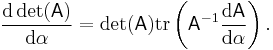
Derivative
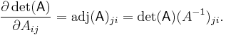
By definition, e.g., using the Leibniz formula, the determinant of real (or analogously for complex) square matrices is a polynomial function from Rn×n to R. As such it is everywhere differentiable. Its derivative can be expressed using Jacobi's formula:
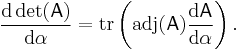
where adj(A) denotes the adjugate of A. In particular, if A is invertible, we have
Expressed in terms of the entries of A, these are
Yet another equivalent formulation is
 ,
,
using big O notation. The special case where  , the identity matrix, yields

This identity is used in describing the tangent space of certain matrix Lie groups.
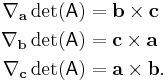
If the matrix A is written as 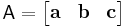 where a, b, c are vectors, then the gradient over one of the three vectors may be written as the cross product of the other two:
Natural transformation
A matrix over a commutative ring R is invertible if and only if its determinant is a unit in R. For a commutative ring R and a natural number n, det is a mapping between GLn(R) (the group of invertible n×n matrices with entries in R) and R× (the group of units in R), making detR (the specialization of det for a concrete commutative ring R) a morphism in the category of groups Grp. The category of commutative rings CRng and Grp are related by two functors GLn and ( )×, where GLn maps any given commutative ring R to the group GLn(R), and ( )× maps any given commutative ring R to the group R×. Every morphism f : R → S in CRng (with R and S being commutative rings) induces corresponding morphisms GLn f : GLn(R) → GLn(S) and f× : R× → S× in Grp, with detS ° GLn f = f× ° detR. Therefore det is a natural transformation between GLn and ( )×.[4]
The above stated more briefly: Let R be a commutative ring. The map 'take-the-determinant' is a morphism of algebraic groups from GLn,R to Gm,R.
Abstract formulation
An n × n square matrix A may be thought of as the coordinate representation of a linear transformation of an n-dimensional vector space V. Given any linear transformation
we can define the determinant of A as the determinant of any matrix representing A. This is a well-defined notion (i.e. independent of a choice of basis) since the determinant is invariant under similarity transformations.
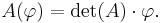
The determinant of a linear transformation A can be formulated in a coordinate-free manner, as follows. The set of alternating multilinear forms ΛnV is a vector space, on which A induces a linear transformation. Given φ ∈ ΛnV, define A(φ) ∈ ΛnV as

Because n is also the dimension of V, ΛnV is one-dimensional and this operation is just multiplication by some scalar that depends on A. This scalar is called the determinant of A. That is, det(A) is defined by the equation
To see that this definition agrees with the coordinate-dependent definition given above, one can use the characterization of the determinant given above: for example switching two columns changes the parity of the determinant; likewise, permuting the vectors in the exterior product v1 ∧ v2 ∧ ... ∧ vn to v2 ∧ v1 ∧ v3 ∧ ... ∧ vn, say, also alters the parity. Minors of a matrix can also be cast in this setting, by considering lower alternating forms ΛkV with k < dim V.
Algorithmic implementation
- The naive method of implementing an algorithm to compute the determinant is to use Laplace's formula for expansion by cofactors. This approach is extremely inefficient in general, however, as it is of order n! (n factorial) for an n×n matrix M.
- An improvement to order n3 can be achieved by using LU decomposition to write M = LU for triangular matrices L and U. Now, det M = det LU = det L det U, and since L and U are triangular the determinant of each is simply the product of its diagonal elements. Alternatively one can perform the Cholesky decomposition if possible or the QR decomposition and find the determinant in a similar fashion.
- If two matrices of order n can be multiplied in time M(n), where M(n)≥na for some a>2, then the determinant can be computed in time O(M(n)).[5] This means, for example, that an O(n2.376) algorithm exists based on the Coppersmith–Winograd algorithm.
- Since the definition of the determinant does not need divisions, a question arises: do fast algorithms exist that do not need divisions? This is especially interesting for matrices over rings. Indeed algorithms with run-time proportional to n4 exist. An algorithm of Mahajan and Vinay, and Berkowitz[6] is based on closed ordered walks (short clow). It computes more products than the determinant definition requires, but some of these products cancel and the sum of these products can be computed more efficiently. The final algorithm looks very much like an iterated product of triangular matrices.
- What is not often discussed is the so-called "bit complexity" of the problem, i.e. how many bits of accuracy you need to store for intermediate values. For example, using Gaussian elimination, you can reduce the matrix to upper triangular form, then multiply the main diagonal to get the determinant (this is essentially a special case of the LU decomposition as above), but a quick calculation will show that the bit size of intermediate values could potentially become exponential. One could talk about when it is appropriate to round intermediate values, but an elegant way of calculating the determinant uses the Bareiss Algorithm, an exact-division method based on Sylvester's identity to give a run time of order n3 and bit complexity roughly the bit size of the original entries in the matrix times n.
History
Historically, determinants were considered without reference to matrices: originally, a determinant was defined as a property of a system of linear equations. The determinant "determines" whether the system has a unique solution (which occurs precisely if the determinant is non-zero). In this sense, determinants were first used in the Chinese mathematics textbook The Nine Chapters on the Mathematical Art (九章算術, Chinese scholars, around the 3rd century BC). In Europe, two-by-two determinants were considered by Cardano at the end of the 16th century and larger ones by Leibniz and, in Japan, by Seki about 100 years later.[7][8][9]
In Japan, determinants were introduced to study elimination of variables in systems of higher-order algebraic equations. They used it to give short-hand representation for the resultant. After the first work by Seki in 1683, Laplace's formula was given by two independent groups of Japanese mathematicians: Tanaka, Iseki (算法発揮, Sampo-Hakki, published in 1690) and Seki, Takebe, Takebe (大成算経, taisei-sankei, written at least before 1710). However, doubts have been raised about how much they recognized the determinant as an independent object.
In Europe, Cramer (1750) added to the theory, treating the subject in relation to sets of equations. The recurrent law was first announced by Bézout (1764).
It was Vandermonde (1771) who first recognized determinants as independent functions.[7] Laplace (1772) [10][11] gave the general method of expanding a determinant in terms of its complementary minors: Vandermonde had already given a special case. Immediately following, Lagrange (1773) treated determinants of the second and third order. Lagrange was the first to apply determinants to questions of elimination theory; he proved many special cases of general identities.
Gauss (1801) made the next advance. Like Lagrange, he made much use of determinants in the theory of numbers. He introduced the word determinants (Laplace had used resultant), though not in the present signification, but rather as applied to the discriminant of a quantic. Gauss also arrived at the notion of reciprocal (inverse) determinants, and came very near the multiplication theorem.
The next contributor of importance is Binet (1811, 1812), who formally stated the theorem relating to the product of two matrices of m columns and n rows, which for the special case of m = n reduces to the multiplication theorem. On the same day (November 30, 1812) that Binet presented his paper to the Academy, Cauchy also presented one on the subject. (See Cauchy-Binet formula.) In this he used the word determinant in its present sense,[12][13] summarized and simplified what was then known on the subject, improved the notation, and gave the multiplication theorem with a proof more satisfactory than Binet's.[7][14] With him begins the theory in its generality.
The next important figure was Jacobi[8] (from 1827). He early used the functional determinant which Sylvester later called the Jacobian, and in his memoirs in Crelle for 1841 he specially treats this subject, as well as the class of alternating functions which Sylvester has called alternants. About the time of Jacobi's last memoirs, Sylvester (1839) and Cayley began their work.[15][16]
The study of special forms of determinants has been the natural result of the completion of the general theory. Axisymmetric determinants have been studied by Lebesgue, Hesse, and Sylvester; persymmetric determinants by Sylvester and Hankel; circulants by Catalan, Spottiswoode, Glaisher, and Scott; skew determinants and Pfaffians, in connection with the theory of orthogonal transformation, by Cayley; continuants by Sylvester; Wronskians (so called by Muir) by Christoffel and Frobenius; compound determinants by Sylvester, Reiss, and Picquet; Jacobians and Hessians by Sylvester; and symmetric gauche determinants by Trudi. Of the text-books on the subject Spottiswoode's was the first. In America, Hanus (1886), Weld (1893), and Muir/Metzler (1933) published treatises.
See also
- Matrix determinant lemma
- Permanent
- Minor (linear algebra)
- Trace (linear algebra)
- Slater determinant
- Pseudo-determinant
Notes
- ↑ Proofs can be found in http://web.archive.org/web/20080113084601/http://www.ee.ic.ac.uk/hp/staff/www/matrix/proof003.html
- ↑ These identities were taken http://www.ee.ic.ac.uk/hp/staff/dmb/matrix/proof003.html
- ↑ Proofs are given at http://www.mth.kcl.ac.uk/~jrs/gazette/blocks.pdf
- ↑ Mac Lane, Saunders (1998), Categories for the Working Mathematician, Graduate Texts in Mathematics 5 ((2nd ed.) ed.), Springer-Verlag, ISBN 0-387-98403-8
- ↑ J.R. Bunch and J.E. Hopcroft, Triangular factorization and inversion by fast matrix multiplication, Mathematics of Computation, 28 (1974) 231–236.
- ↑ http://page.inf.fu-berlin.de/~rote/Papers/pdf/Division-free+algorithms.pdf
- ↑ 7.0 7.1 7.2 Campbell, H: "Linear Algebra With Applications", pages 111-112. Appleton Century Crofts, 1971
- ↑ 8.0 8.1 Eves, H: "An Introduction to the History of Mathematics", pages 405, 493–494, Saunders College Publishing, 1990.
- ↑ A Brief History of Linear Algebra and Matrix Theory : http://darkwing.uoregon.edu/~vitulli/441.sp04/LinAlgHistory.html
- ↑ Expansion of determinants in terms of minors: Laplace, Pierre-Simon (de) "Researches sur le calcul intégral et sur le systéme du monde," Histoire de l'Académie Royale des Sciences (Paris), seconde partie, pages 267-376 (1772).
- ↑ Muir, Sir Thomas, The Theory of Determinants in the historical Order of Development [London, England: Macmillan and Co., Ltd., 1906].
- ↑ The first use of the word "determinant" in the modern sense appeared in: Cauchy, Augustin-Louis “Memoire sur les fonctions qui ne peuvent obtenir que deux valeurs égales et des signes contraires par suite des transpositions operées entre les variables qu'elles renferment," which was first read at the Institute de France in Paris on November 30, 1812, and which was subsequently published in the Journal de l'Ecole Polytechnique, Cahier 17, Tome 10, pages 29-112 (1815).
- ↑ Origins of mathematical terms: http://jeff560.tripod.com/d.html
- ↑ History of matrices and determinants: http://www-history.mcs.st-and.ac.uk/history/HistTopics/Matrices_and_determinants.html
- ↑ The first use of vertical lines to denote a determinant appeared in: Cayley, Arthur "On a theorem in the geometry of position," Cambridge Mathematical Journal, vol. 2, pages 267-271 (1841).
- ↑ History of matrix notation: http://jeff560.tripod.com/matrices.html
References
- Axler, Sheldon Jay (1997), Linear Algebra Done Right (2nd ed.), Springer-Verlag, ISBN 0387982590
- de Boor, Carl (1990), "An empty exercise", ACM SIGNUM Newsletter 25 (2): 3–7, doi:10.1145/122272.122273, http://ftp.cs.wisc.edu/Approx/empty.pdf.
- Lay, David C. (August 22, 2005), Linear Algebra and Its Applications (3rd ed.), Addison Wesley, ISBN 978-0321287137
- Meyer, Carl D. (February 15, 2001), Matrix Analysis and Applied Linear Algebra, Society for Industrial and Applied Mathematics (SIAM), ISBN 978-0898714548, http://www.matrixanalysis.com/DownloadChapters.html
- Poole, David (2006), Linear Algebra: A Modern Introduction (2nd ed.), Brooks/Cole, ISBN 0-534-99845-3
- Anton, Howard (2005), Elementary Linear Algebra (Applications Version) (9th ed.), Wiley International
- Leon, Steven J. (2006), Linear Algebra With Applications (7th ed.), Pearson Prentice Hall
External links
- Linear Systems Chapter from "Fundamental Problems of Algorithmic Algebra" Chee Yap's chapter on Linear Systems describing implementation aspects of Determinant computation.
- Mahajan, Meena and V. Vinay, “Determinant: Combinatorics, Algorithms, and Complexity”, Chicago Journal of Theoretical Computer Science, v. 1997 article 5 (1997).
- Online Matrix Calculator Online Matrix calculator.
- Linear algebra: determinants. Compute determinants of matrices up to order 6 using Laplace expansion you choose.
- Matrices and Linear Algebra on the Earliest Uses Pages
- Determinants explained in an easy fashion in the 4th chapter as a part of a Linear Algebra course.
- Instructional Video on taking the determinant of an nxn matrix (Kahn Academy)