Median
In probability theory and statistics, a median is described as the numeric value separating the higher half of a sample, a population, or a probability distribution, from the lower half. The median of a finite list of numbers can be found by arranging all the observations from lowest value to highest value and picking the middle one. If there is an even number of observations, then there is no single middle value; the median is then usually defined to be the mean of the two middle values.[1][2]
In a sample of data, or a finite population, there may be no member of the sample whose value is identical to the median (in the case of an even sample size) and, if there is such a member, there may be more than one so that the median may not uniquely identify a sample member. Nonetheless the value of the median is uniquely determined with the usual definition. A related concept, in which the outcome is forced to correspond to a member of the sample is the medoid.
At most half the population have values less than the median and at most half have values greater than the median. If both groups contain less than half the population, then some of the population is exactly equal to the median. For example, if a < b < c, then the median of the list {a, b, c} is b, and if a < b < c < d, then the median of the list {a, b, c, d} is the mean of b and c, i.e. it is (b + c)/2.
The median can be used as a measure of location when a distribution is skewed, when end values are not known, or when one requires reduced importance to be attached to outliers, e.g. because they may be measurement errors. A disadvantage of the median is the difficulty of handling it theoretically.
Notation
The median of some variable x is denoted either as  or as
or as  [3]
[3]
Measures of statistical dispersion
When the median is used as a location parameter in descriptive statistics, there are several choices for a measure of variability: the range, the interquartile range, the mean absolute deviation, and the median absolute deviation. Since the median is the same as the second quartile, its calculation is illustrated in the article on quartiles.
Medians of probability distributions
For any probability distribution on the real line with cumulative distribution function F, regardless of whether it is any kind of continuous probability distribution, in particular an absolutely continuous distribution (and therefore has a probability density function), or a discrete probability distribution, a median m satisfies the inequalities
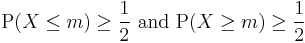
or
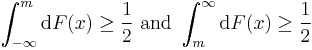
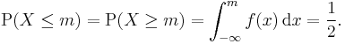
in which a Lebesgue–Stieltjes integral is used. For an absolutely continuous probability distribution with probability density function ƒ, we have
Medians of particular distributions
The medians of certain types of distributions can be easily calculated from their parameters: The median of a normal distribution with mean μ and variance σ2 is μ. In fact, for a normal distribution, mean = median = mode. The median of a uniform distribution in the interval [a, b] is (a + b) / 2, which is also the mean. The median of a Cauchy distribution with location parameter x0 and scale parameter y is x0, the location parameter. The median of an exponential distribution with rate parameter λ is the natural logarithm of 2 divided by the rate parameter: λ−1ln 2. The median of a Weibull distribution with shape parameter k and scale parameter λ is λ(ln 2)1/k.
Medians in descriptive statistics
The median is primarily used for skewed distributions, which it summarizes differently than the arithmetic mean. Consider the multiset { 1, 2, 2, 2, 3, 14 }. The median is 2 in this case, as is the mode, and it might be seen as a better indication of central tendency than the arithmetic mean of 4.
Calculation of medians is a popular technique in summary statistics and summarizing statistical data, since it is simple to understand and easy to calculate, while also giving a measure that is more robust in the presence of outlier values than is the mean.
Theoretical properties
An optimality property
A median is also a central point which minimizes the average of the absolute deviations. In the above example, the median value of 2 minimizes the average of the absolute deviations (1 + 0 + 0 + 0 + 1 + 12) / 6 = 2.33; in contrast, the mean value of 4 minimizes the average of the squares (9 + 4 + 4 + 4 + 1 + 100) / 6 = 20.33. In the language of statistics, a value of c that minimizes

is a median of the probability distribution of the random variable X.
However, a median c need not be uniquely defined. Where exactly one median exists, statisticians speak of "the median" correctly; even when no unique median exists, some statisticians speak of "the median" informally.
An inequality relating means and medians
For continuous probability distributions, the difference between the median and the mean is less than or equal to one standard deviation. See an inequality on location and scale parameters.
The sample median
Efficient computation of the sample median
Even though sorting n items generally requires O(n log n) operations, the median of n items can be computed with only O(n) operations. In fact, one can always find the kth smallest of n items with a O(n)-operations selection algorithm.
Easy explanation of the sample median
For an odd number of values
As an example, we will calculate the sample median for the following set of observations: 1, 5, 2, 8, 7.
Start by sorting the values: 1, 2, 5, 7, 8.
In this case, the median is 5 since it is the middle observation in the ordered list.
For an even number of values
As an example, we will calculate the sample median for the following set of observations: 1, 5, 2, 8, 7, 2.
Start by sorting the values: 1, 2, 2, 5, 7, 8.
In this case, the average of the two middlemost terms is (2 + 5)/2 = 3.5. Therefore, the median is 3.5 since it is the average of the middle observations in the ordered list.
Other estimates of the median
If data are represented by a statistical model specifying a particular family of probability distributions, then estimates of the median can be obtained by fitting that family of probability distributions to the data and calculating the theoretical median of the fitted distribution. See, for example Pareto interpolation.
Median-unbiased estimators, and bias with respect to loss functions
Any mean-unbiased estimator minimizes the risk (expected loss) with respect to the squared-error loss function, as observed by Gauss. A median-unbiased estimator minimizes the risk with respect to the absolute-deviation loss function, as observed by Laplace. Other loss functions are used in statistical theory, particularly in robust statistics.
The theory of median-unbiased estimators was revived by George W. Brown in 1947:
An estimate of a one-dimensional parameter θ will be said to be median-unbiased, if for fixed θ, the median of the distribution of the estimate is at the value θ, i.e., the estimate underestimates just as often as it overestimates. This requirement seems for most purposes to accomplish as much as the mean-unbiased requirement and has the additional property that it is invariant under one-to-one transformation. [page 584]
Further properties of median-unbiased estimators have been noted by Lehmann, Birnbaum, van der Vaart and Pfanzagl. In particular, median-unbiased estimators exist in cases where mean-unbiased and maximum-likelihood estimators do not exist. Besides being invariant under one-to-one transformations, median-unbiased estimators have surprising robustness.
In image processing
In monochrome raster images there is a type of noise, known as the salt and pepper noise, when each pixel independently become black (with some small probability) or white (with some small probability), and is unchanged otherwise (with the probability close to 1). An image constructed of median values of neighborhoods (like 3×3 square) can effectively reduce noise in this case.
In multidimensional statistical inference
In multidimensional statistical inference, the value  that minimizes
  is also called a centroid.[4] In this case
  is indicating a norm for the vector difference, such as the Euclidean norm, rather than the one-dimensional case's use of an absolute value. (Note that in some other contexts a centroid is more like a multidimensional mean than the multidimensional median described here.)
Like a centroid, a medoid minimizes , but is restricted to be a member of specified set. For instance, the set could be a sample of points drawn from some distribution.
History
Gustav Fechner popularized the median into the formal analysis of data, although it had been used previously by Laplace.[5]
See also
- Order statistic
- Quantile
- A median is the 2nd quartile, 5th decile, and 50th percentile.
- A sample-median is median-unbiased but can be a mean-biased estimator.
- Absolute deviation
- Concentration of measure for Lipschitz functions
- An inequality on location and scale parameters
- Median voter theory
- Median graph
- The centerpoint is a generalization of the median for data in higher dimensions.
- Median search
- Hinges
References
- ↑ http://mathworld.wolfram.com/StatisticalMedian.html Weisstein, Eric W. "Statistical Median." From MathWorld--A Wolfram Web Resource. http://mathworld.wolfram.com/StatisticalMedian.html
- ↑ http://www.stat.psu.edu/old_resources/ClassNotes/ljs_07/sld008.htm Simon, Laura J "Descriptive statistics" Statistical Education Resource Kit Penn State Department of Statistics
- ↑ http://mathworld.wolfram.com/StatisticalMedian.html
- ↑ Carvalho, Luis; Lawrence, Charles (2008), "Centroid estimation in discrete high-dimensional spaces with applications in biology", Proc Natl Acad Sci U S A 105 (9): 3209–3214, doi:10.1073/pnas.0712329105
- ↑ Keynes, John Maynard; A Treatise on Probability (1921), Pt II Ch XVII §5 (p 201).
- Brown, George W. ”On Small-Sample Estimation.” The Annals of Mathematical Statistics, Vol. 18, No. 4 (Dec., 1947), pp. 582–585.
- Lehmann, E. L. “A General Concept of Unbiasedness” The Annals of Mathematical Statistics, Vol. 22, No. 4 (Dec., 1951), pp. 587–592.
- Allan Birnbaum. 1961. “A Unified Theory of Estimation, I”, The Annals of Mathematical Statistics, Vol. 32, No. 1 (Mar., 1961), pp. 112–135
- van der Vaart, H. R. 1961. “Some Extensions of the Idea of Bias” The Annals of Mathematical Statistics, Vol. 32, No. 2 (Jun., 1961), pp. 436–447.
- Pfanzagl, Johann; with the assistance of R. Hamböker (1994). Parametric Statistical Theory. Walter de Gruyter. ISBN 3-11-01-3863-8. MR1291393
External links
- A Guide to Understanding & Calculating the Median
- Median as a weighted arithmetic mean of all Sample Observations
- On-line calculator
- Calculating the median
- A problem involving the mean, the median, and the mode.
- mathworld: Statistical Median
- Python script for Median computations and income inequality metrics
This article incorporates material from Median of a distribution on PlanetMath, which is licensed under the Creative Commons Attribution/Share-Alike License.
|
|||||||||||||||||||||||||||||||||||||||||||||||||||||||||||||||||||||||||||||||||||||||||||||||||||||||||||||||||||||||||||||||||||||||||